The system grew out of an interface and over 30 modules for handling multicomponent data that I wrote for DISCO on VAX 11/789 between 1993 - 1995. Due to this heritage, SIA still supports a simple job description language close to that of DISCO and can include modules written for DISCO practicaly without any modifications. However, every bit of the system package and every module were written from scratch based on a significantly broader concept of seismic processing than that usually employed by commercial developers. In its software implementation, an object-oriented approach allowed creation of a flexible and scaleable system.
The SIA system is designed for a broad range of seismic processing applications. Its distinctive features are generic support of complexly structured data flows and flexible parameter input. The basic data structure in the system is not a trace or even a trace nsemble, but a trace ensemble sequence (multicomponent, optionally 3-D trace gather), with all auxiliary information attached to the traces and ensembles in a natural way. This makes the system highly suitable for processing of multicomponent datasets.
Compared to data handling in Seismic UNIX and in commercial processing systems, SIA has a number of important advantages:
The most basic data structures - traces and database tables, - are supported by the core of the system. The only difference between traces and other data structures that traces are "pulled" through the processing flow during the so-called "Process phase" while all of the other objects are generated and destroyed by the tools, and recognized by their names. Otherwise, these data types are similar; for example, database tables can be treated as traces and propagated through the processing modules.
As the system grows, new modules introduce additional data types, such as velocity or gravity models, images, artificial neural networks, etc. These data objects are maintained entirely by these modules, and thus no modifications of the monitor are required in order to incorporate new processing packages.
Although called "traces", the basic data units in the system are no longer fixed-length arrays. "Traces" can be two-or three-dimensional grids, f-k or t-p spectra, spectrograms (see spctrgr) graphic images, and arbitrary memory blocks. Every trace consists of a data segment of an arbitrary length and of a header. Data segments consist of several (usually 1) records. Even within one ensemble, traces can be of different lengths and formats.
Trace header consists of an arbitrary number of entries. Every entry is of one of the following formats: INTEGER (32-bit integer), LONG (64-bit integer), FLOAT (32-bit), DOUBLE (64-bit), and CHARACTER of an arbitrary length. The number of data samples, sample interval, and the trace header format may vary from one module to another. Traces may have a non-zero time start (trace header entry TIMSTRT). For example, processing a wide-angle data set, it is convenient to store the traces in a time-reduced form, saving up to 50% of disk storage and CPU time.
Vital trace information is stored in predefined trace headers (TIMSTRT above is just one example). These headers can be accessed directly as well as through methods of C++ objects TRACE, ENSEMBLE, and GATHER.
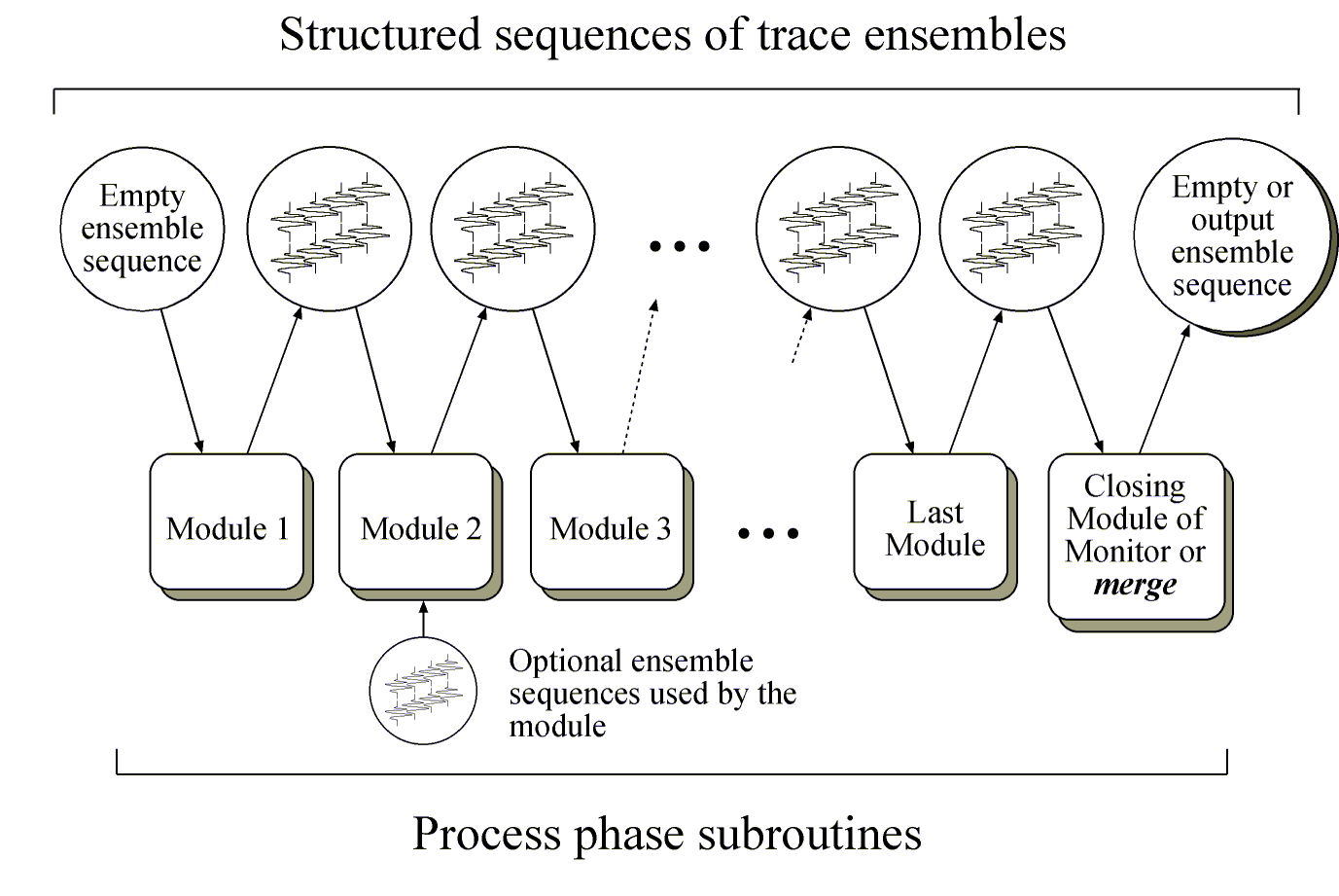
Internally, each processing module always "sees" two structured sequences of trace ensembles, one of them at the module's input and the second—at the output (Figure 1). Ensembles are interconnected sequences of traces, typically (but not necessarily!) ended with a trace having the value of a predefined trace header LASTTR=1. A natural example of a trace ensemble is a set of records simultaneously acquired by a multicomponent instrument. Every module has standard input and output ensemble sequences (Figure 1). However, the modules can create their own ensemble sequences (Figure 1), and some named ensemble sequences can be created by the user so that they are accessible to all modules (see modules store and load).

SIA supports a variety of system-wide databases existing independently of current data flow. These databases are loosely referred as tables. Tables can be viewed as sorted sequences of trace headers without data samples. The entire sequences of table records can be generated, processed and removed during Edit and Process phases.
Tables are recognized by their symbolic names specified by the user, and user-defined formats. Once loaded, tables are visible to all modules in the same job, and many tables can be used in one job. A number of modules allow creation and modifications of tables, mathematical operations with their entries, plotting of the values, and exchange of the data between tables and trace headers. Travel time processing package is implemented using manipulations with tables. Modules readtab and pritab convert tables from and to ASCII format. Savetab and loadtab provide means for fast table storage and retrieval from binary files, with an arbitrary number of tables stored in each file.
Starting in version 2.1, modules write and dskrd are able to save and retrieve tables from the same files in which data traces are stored. This feature is useful to maintain any dataset-dependent auxiliary information.
Two table formats are defined, and many modules can work with both formats. In both formats, tables contain an arbitrary number of argument header entries and dependent header entries, called simply entries. All table entries have structures identical to those of trace header entries—with symbolic names and formats as described above.
The main free-table format is referred simply as TABLE (see the description of module readtab). In this format, all argument entries are sorted in the order of increasing values of the first argument. If the argument is a floating-point value, its values are compared with a certain tolerance, and thus the values lying in a certain range are considered to be equal3. All entries with the same value of the first argument are sorted by the increasing values of the second argument, etc.
In the second table format, MAP, the table represents a multidimensional array of multi-entry records. The arguments assume arbitrary but fixed values for all rows (columns, etc.) of the array; these values are listed in the table header. This type of table structure is mostly used to implement functions in multidimensional spaces, such as 2-D or 3-D velocity models or travel-time maps defined on irregular rectangular grids.
All modules in a job can access a common set of parameters that are referred as "job parameters". Normally, these parameters can be used anywhere a numeric value is expected. Internally, these parameters are formatted as a trace header, and thus many operations associated with trace headers can be performed on this parameter area. The parameters are identified by their names, and mathematical operations can be performed on them using module parmath. Job parameters allow to implement a more elaborate parameterization than it is possible with simple text substitutions. For example, one can supply a phase value, say, phi, through the command line (see *params), and to ensure that another two variables are always equal sin(phi) and cos(phi).